Analytical methods: Maximum Likelihood
Model-based methods
The maximum likelihood aproach shares a great deal with parsimony, but it uses a different optimality criterion.
In maximum likelihood, the tree that is most likely to have given rise to the observed data is considered best.
To determine this likelihood, it is necessary to use a probabilistic model of sequence (i.e., character-state) evolution.
Parsimony assumes that homoplasy (character-state reversal) is rare, but does not make use of explicit probabilistic models. With certain data types, particularly those with a limited number of character states, the assumption that homoplasy is rare can be shown to be violated.
Maximum Likelihood
What is Likelihood?
Probability refers to the chance of drawing things from a defined
population
But many abstract concepts, like evolutionary trees, don't draw
from a defined and finite population.
Thus probability per se can't apply.
Likelihood is proportional to probability, but the ratio of proportion
is arbitrary.
L(H|R) -- the likelihood of a hypothesis "H" given a set of data
"R" proportional to a conditional probability P(H|R).
The model relates the hypothesis (tree) to the data (sequences)
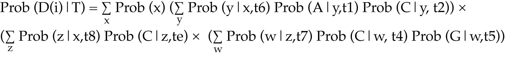
Calculating the likelihood of a tree
Given a tree with branch lengths
For each character, assign the appropriate character state to the tips of the tree
Sum the probabilities of all possible ancestral states
This gives a site likelihood, i.e., the likelihood for that character, or site within the sequence
This is the likelihood of observing those character states given the tree
To calculate these site likelihoods, it is necessary to know the probability of character-state change over time. We will discuss models of character-state evolution shortly.

This sum is a likelihood because all possible terminal character states are not considered; the calculations only reflect those that are present in the dataset.
Computing the site likelihoods efficiently relies on calculating conditional likelihoods for sub-trees
Start at a node where all of the descendant nodes are tips on the tree. Ignoring ambiguity and missing data for the time being, the tips will all have a known character-state, and consequently will have a likelihood of 1 for that character-state.
For that node, calculate the likelihood of each of the four character-states.
Assuming the branches are of finite length, even nodes with descendents that have the same character state will have a non-zero likelihood for each of the other possible character-states.
Recursively calculate the likelihood of the character-states for each of the nodes moving down the tree.
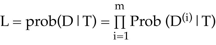
The tree likelihood is the product of all of the site likelihoods
This is the likelihood of the entire dataset given the tree
To make calculation easier, most implementations convert site likelihoods to logarithms, and then sum the log likelihoods.
This likelihood is very small; this reflects the fact that the observed sequence alignment is only one of many that could have resulted, given the tree.
Models of character-state change
Evolution of a two-state system
Assume character state changes are independent
The past states held by a given site (character) do not change the future states it can hold
This is a Markov model
The probability of character state change is a function of time and rate of change. This value (time x rate) is the branch length.
DNA sequence evolution
Jukes-Cantor
Four possible character states
All substitutions are equally likely
All nucleotides occur with equal frequency
Kimura two-parameter
Transition-transversion ratio
-
| |
A |
C |
G |
T |
| A |
|
Transversion |
Transition |
Transversion |
| C |
Transversion |
|
Transversion |
Transition |
| G |
Transition |
Transversion |
|
Transversion |
| T |
Transversion |
Transition |
Transversion |
|
In the evolution of real sequences transitions are typically observed
more often than transversions.
Example of a substitution probability matrix consistent with the K2P model.
| |
A |
C |
G |
T |
| A |
0.6 |
0.1 |
0.2 |
0.1 |
| C |
0.1 |
0.6 |
0.1 |
0.2 |
| G |
0.2 |
0.1 |
0.6 |
0.1 |
| T |
0.1 |
0.2 |
0.1 |
0.6 |
These values represent the probability of the corresponding event occurring
within a unit of time, t.
The values in the diagonals are selected such that each row adds up
to one. Each row has to add up to one because the substitution matrix
takes into account all possible events within the model.
Felsenstein, Chapters 9 & 16
Hillis, Moritz & Mable, pp. 426-446
Felsenstein, J. 1978. Cases in which parsimony or compatibility methods will
be positively misleading. Systematic Zoology 27: 401-410.
Li, W.-H. 1997. Molecular Evolution. Sinauer Associates, Inc., Sunderland,
MA. Pp. 116-119.